Python coding

OpenCV basics

last updated: 2020-12-06

Installation

For more infos on installing Python look here.

The modules can be are installed with pip:

    pip install opencv-python
    pip install pandas

Read an image and show it

With the function cv2.imread() we read an image. The first argument will be the image name (string). The image should be in the working directory or a full path of image must be given. The second argument is one of the following flags which specifies the way the image should be read.

cv.IMREAD_COLOR:
RGB colour image. Any transparency of image will be neglected. It is the default flag.
cv.IMREAD_GRAYSCALE:
Image is loaded in greyscale mode
cv.IMREAD_UNCHANGED:
Loads image including alpha channel (transparency)

Many image formats are supported (bmp, pbm, pgm, ppm, sr, ras, jpeg, jpg, jpe, tiff, tif, png).

To show the image we need beneath the cv.imshow() function two other functions to wait, so that the picture can be seen for a certain time and to close the image show.

The cv.waitKey(0) function waits for a key to be pressed, or a certain amount of time in ms if the argument is not zero and cv.destroyAllWindows() closes the show.

Minimal program

Here is a minimal program:

    import cv2 as cv

    IMG_NAME = 'test.jpg'
    img = cv.imread(IMG_NAME)      # read the image (default RGB colour no alpha)
    cv.imshow('image', img)        # cv.imshow(window_name, image)
    cv.waitKey(0)                  # show picture til keypressed
    cv.destroyAllWindows()

Example using a function and showing all images from a directory

As always three commands are needed to show an image, it is a good idea to write a function. The following code displays png and jpg-images stored in a directory. The function gets as second argument a tuple (2 values). The first value is a flag, defining if the picture should be displayed (1) or not (0). The second value is the time in ms (or 0 to wait on a key to be pressed). With a dictionary or a list it is possible to define multiple tuples and change the behaviour of the program.

    #!/usr/bin/python3
    # -*- coding: utf-8 -*-
    """ Program to read and show images from a folder """

    import os
    import glob
    import cv2 as cv                      # to run code even if version changes

    DIR_NAME_IMAGES = '/savit/programming/python/opencv/images'

    def show_image(pimg, show_flag_time):
        ''' Show image during x ms if flag is set. Parameter show_flag_time is a
            tuple e.g (1,2000) to show picture for 2s or (0,2000) to prevent the
            show. (1,0) waits on keypress '''
        if show_flag_time[0] == 1:
            cv.imshow('image', pimg)      # cv.imshow(window_name, image)
            cv.waitKey(show_flag_time[1]) # show picture for x ms (x=0 for keypress)
            cv.destroyAllWindows()

    # flags and times in ms to show images
    flag = {'short':(1, 500), 'medium':(1, 1000), 'long':(1, 3000), 'key':(1,0)}

    os.chdir(DIR_NAME_IMAGES)             # change directory
    img_list = glob.glob('*.jpg')         # get list with jpg images
    img_list.extend(glob.glob('*.png'))   # and png images
    img_list.sort()                       # sort the list
    print(img_list)
    if img_list == []:
        print("error: no images!")

    i = 0
    for img_name in img_list:
        i += 1
        img = cv.imread(img_name)         # read the image
        show_image(img, flag[str(i)])

Working with images

Let's take a closer look at an image. An image opened with OpenCV is saved as a two (grey) or three dimensional numpy array (colour).

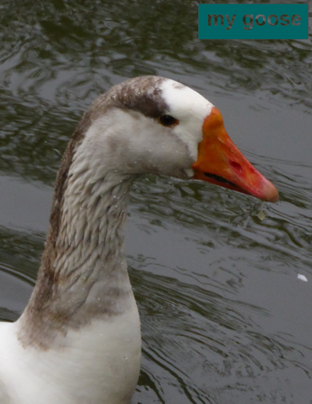
We will use the test.jpg image from the Download section (bottom of the page).

Get dimensions

First we want to know the dimensions. For this we can use the shape method that returns the height, width and the number of channels as a tuple. For a coloured picture we get 3 colours (BGR). The dtype method shows that every colour uses one byte (0-255).

The origin of images is top left.

    flag = {'short':(1, 500), 'medium':(1, 1000), 'long':(1, 3000)}

    img = cv.imread(IMG_NAME)                        # read the image
    show_image(img, flag['medium'])
    print(img.shape, image.type)                     # shape returns height,width,channels
    height, width = img.shape[:2]
    print("height x width = ", height, 'x', width)

    height x width =  1500 x 2000

Now let's look at the firs 4 pixel top left. BRG numbers are close together, so we get as colour some light grey.

    img_pixel = img[0:2, 0:2]
    show_image(img_pixel, flag['medium'])
    print(img_pixel)                                 # print 4 pixel (2x2)

    [[[88 91 95]
      [86 89 93]]
     [[90 93 97]
      [86 89 93]]]

Reduce size and write image to file

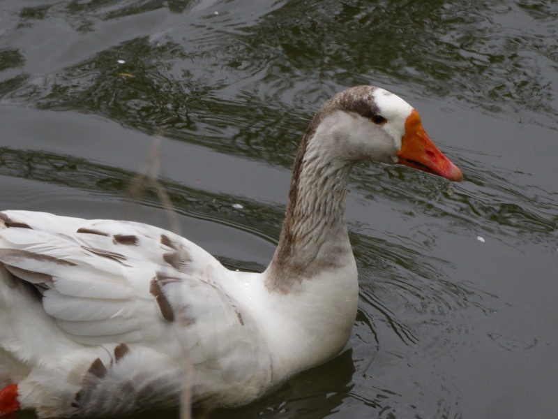
With the resize() method we can down or upscale an image. The first parameter is the image, the second patrameter the wanted dimensions (x,y). If we set the dimensions to (0,0) we can use the optional scale factors fx and fy.

With the imwrite() method we write the image to a file. First parameter is the image nameand the seconf parameter the image. In this example we use the old image name and the find() method to add text to the image name.

scan down or upscale an image. The first parameter

    RATIO = 0.4
    r_img = cv.resize(img, (0, 0), fx=ratio, fy=ratio)
    show_image(r_img, flag['medium'])
    cv.imwrite(IMG_NAME[0:IMG_NAME.find('.')] + '_40p.jpg', r_img)   # write r_img
    print("height x width = ", r_img.shape[0], 'x', r_img.shape[1])

    height x width =  600 x 800

Creating a copy

This is straightforward by using the copy() method:

    imgc = r_img.copy()                              # copy of an image
    show_image(imgc, flag['medium'])

Cropping (slicing), copying parts and setting pixels

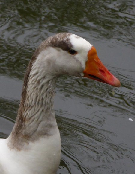
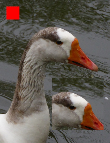
Slicing in Python allows us to cut out or copy any section in an image or to e.g. change the colour of a section.

    img2 = img[100:1200, 900:1750]                   # new image (img2) crop from img
    show_image(img2, flag['medium'])
    img2[50:150, 50:150] = [0, 0, 255]               # BGR: set pixels to red
    show_image(img2, flag['medium'])
    img2[600:1000, 400:800] = img[200:600, 1200:1600]# copy an image part to another image
    show_image(img2, flag['medium'])

Create an image

Let's first create a 2x2 pixel image. A list can be converted to an numpy array with np.asarray().

OpenCV uses the BGR color space. With cvtColor() we can convert an image from one color space to another. There are more than 150 color-space conversion methods available in OpenCV. Let's try COLOR_BGR2RGB and COLOR_BGR2GRAY)

    img3_list = [[[0, 0, 255], [255, 0, 0]], [[0, 0, 0], [255, 255, 255]]]
    img3 = np.asarray(img3_list, dtype=np.uint8)    #create image (np.array) from list
    show_image(img3, flag['medium'])
    img4 = cv.cvtColor(img3, cv.COLOR_BGR2RGB)      # change from BGR to RGB
    show_image(img4, flag['medium'])
    img5 = cv.cvtColor(img3, cv.COLOR_BGR2GRAY)     # change from BGR to GREY
    show_image(img5, flag['medium'])
    img6 = np.zeros([300, 300, 3], dtype=np.uint8)  # create 512*512 black image
    img6.fill(255)                                  # change to white
    show_image(img6, flag['medium'])

Drawing with OpenCV

The OpenCV drawing methods are straightforward. For the line we need after the image parameter, the beginning point ((x₁, y₁) touple), the ending point ((x₂, y₂) touple), the colour (BGR touple) and the line thickness. Similar for the rectangle. For the circle we need the center point and the radius.

It is also possible to use the Matplotlib library (module) to draw to images. Matplotlib uses RGB colour space.

    height, width = img6.shape[:2]
    cv.line(img6, (10, 10), (290, 290), (255, 0, 0), 8)                 # draw line
    show_image(img6, flag['medium'])
    cv.rectangle(img6, (50, 50), (250, 250), (255, 0, 255), 4)          # draw rect.
    show_image(img6, flag['medium'])
    cv.circle(img6, (int(height/2), int(width/2)), 120, (0, 0, 255), 2) # circle
    show_image(img6, flag['medium'])

Thresholding

With the threshold() method we we are able to separate objects in pictures. First we need a greyscale image (first parameter). Each pixel intensity value is compared with a threshold (second parameter TRESH). This value (0-255) ranges from black (0) to white (255) and has to be set to best resolve our wishes. If the pixel value is below the threshold value is set to black (0), otherwise to MAX_VALUE defined in the third parameter. The forth parameter can be one of the following:

cv.THRESH_BINARY
cv.THRESH_BINARY_INV
cv.THRESH_TRUNC
cv.THRESH_TOZERO
cv.THRESH_TOZERO_INV

    LOGO_NAME = 'logo.png'
    THRESH = 65 
    MAX_VALUE = 255

    logo = cv.imread(LOGO_NAME)                        # read the image
    show_image(logo, flag['short'])
    logo_grey = cv.cvtColor(logo, cv.COLOR_BGR2GRAY)      # OpenCV uses BGR
    show_image(logo_grey, flag['short'])
    ret, logo_mask = cv.threshold(logo, THRESH, MAX_VALUE, cv.THRESH_BINARY)
    show_image(logo_mask, flag['medium'])
    ret, logo_mask_inv = cv.threshold(logo_grey, THRESH, MAX_VALUE, cv.THRESH_BINARY_INV)
    show_image(logo_mask_inv, flag['medium'])

By looking at our grey picture we see that it is important to find the right threshold value. The lighter grey has a value of 60 and the darker grey of 70, so a threshold between this values is ok.

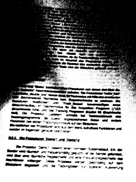
Sometimes normal thresholding is not the best way. Here adaptive thresholding with cv.adaptiveThreshold() can help:

    IMG_NAME_2 = 'test2.png'
    THRESH = 50 
    MAX_VALUE = 255

    img2 = cv.imread(IMG_NAME_2)
    img2_grey = cv.cvtColor(img2, cv.COLOR_BGR2GRAY)
    res, img2_thresh = cv.threshold(img2_grey, THRESH, MAX_VALUE, cv.THRESH_BINARY)
    show_image(img2_thresh, flag['medium'])
    img2_thresh_gauss = cv.adaptiveThreshold(img2_grey,255,cv.ADAPTIVE_THRESH_GAUSSIAN_C,cv.THRESH_BINARY,31,8)
    show_image(img2_thresh_gauss, flag['medium'])

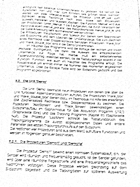
Also it is sometimes usefull to blur the image with cv.medianBlur() before using the threshold() method.

    img_grey_blurred = cv.medianBlur(img_grey,5)

Working with masks

With the threshold method we have already created two masks:

We want to add our logo to an image:

Black (0) is false, every other colour is true. Now we can use bitwise Boolean logic to achieve our goal. To know the dimensions of our logo we use the shape method. Then we define the area in our picture where we want to place the logo and get this part of the image. A bitwise AND (&) with the inverted mask sets the pixels in the black area to 0b00000000 (0 & x = 0) and gets us the background image.

    print(logo.shape, logo.dtype)                      # shape returns height,width,channels
    logo_field = img[10:logo.shape[0]+10, 840-logo.shape[1]:840]
    logo_bg = cv.bitwise_and(logo_field, logo_field, mask=logo_mask_inv)

&

=

Next we use the same procedure on our logo to get the foreground image:

    logo_fg = cv.bitwise_and(logo, logo, mask=logo_mask)

&

=

Now we can add the foreground picture to the background picture an paste the result into the main picture:

    logo_new = cv.add(logo_fg, logo_bg)
    img[10:logo.shape[0]+10, 840-logo.shape[1]:840] = logo_new

+

=

Filtering

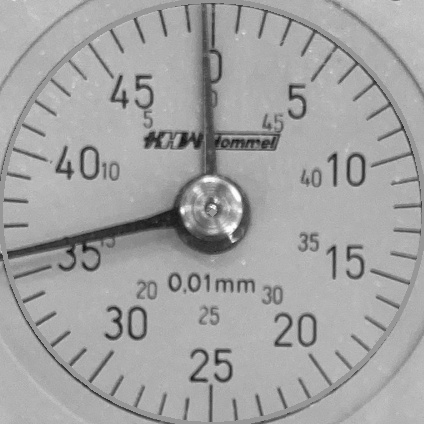
We have the following image and want to retrieve the red hand.

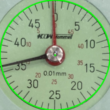
One possibility would be using thresholding. But as we have here a unique colour for the object we will try filtering. To filter we will use the HSV colour scheme. It is much easier to filter with this scheme than with RGB.

HSV stands for Hue, Saturation and Value. Hue defines the colour, the Saturation defines the "colorfulness" of the colour and Value is the Brightness of the colour.

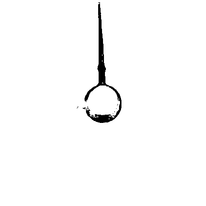
We define the minimum and maximum borders for our colour in numpy arrays. The Hue for the red colour will be between 0 and 10. The Saturation will start only at 60 to eliminate all greyish tones. Brightness goes over the full range(0-255). The method cv.inRange() gives us a black and white image with the red object in white. Here a function that does the work and returns the inverted image:

def get_red(pimg):
    '''filter the red channel'''
    img_hsv = cv.cvtColor(pimg, cv.COLOR_BGR2HSV)
    red_min = np.array([0, 60, 0])
    red_max = np.array([10, 255, 255])
    mask = cv.inRange(img_hsv, red_min, red_max)    
    return ~mask     #return inverted image

Getting lines with cv.HoughLinesP()

The Hough Line Transform is a transform used to detect straight lines. More infos in the OpenCV docs or here.

OpenCV can use the Standard Hough Transform (result is a a vector of couples (θ,rθ)) and the Probabilistic Hough Line Transform. This will be used here, It is more efficient and outputs directly the extremes of the detected lines (x0,y0,x1,y1).

To use the transform we need a grey image and an edge detection pre-processing with the `cv.Canny()`` method is desirable.

    img = cv.imread(IMG_NAME)                        # read the image
    img_grey = cv.cvtColor(img,cv.COLOR_BGR2GRAY)
    img_edges = cv.Canny(img_grey,50,150,apertureSize = 3)
    lines = cv.HoughLinesP(image=img_edges, rho=3, theta=np.pi/180,
                          threshold=100, minLineLength=100, 
                          maxLineGap=30)
    if lines is not None:
        for line in lines: # create image with lines        
            mx1, my1, mx2, my2 = line[0]
            cv.line(img, (mx1, my1), (mx2, my2), (0, 255, 255), 2)        
    show_image(img, flag['key'])

In our picture it would be difficult to get the red hand with this method even by refining the parameters. Here the output for a minLineLength=100 and minLineLength=200:

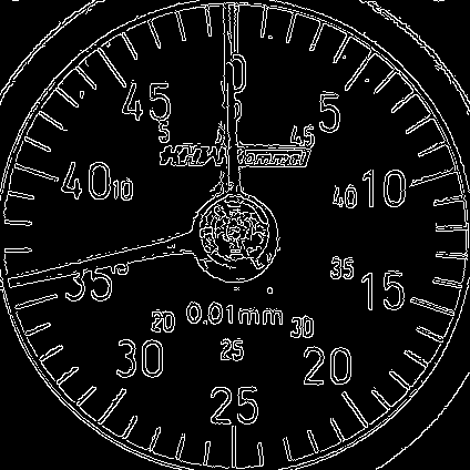
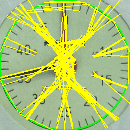
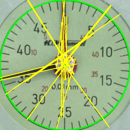
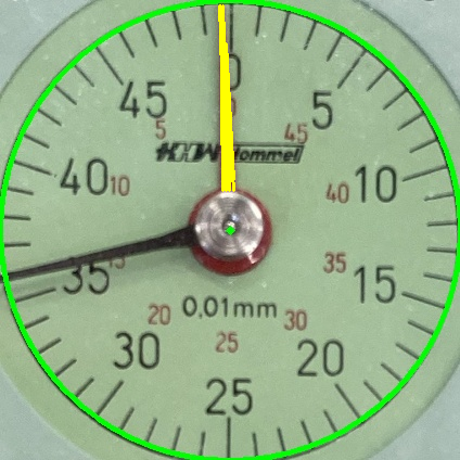
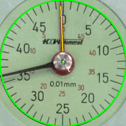
The problem is the second hand in black. Our filtering above (red colour) gives us an image in black and white. We don't need the cv.Canny() function and can directly apply the cv.HoughLinesP() function. By calculating the an average line we get our hand:

    img = cv.imread(IMG_NAME)                        # read the image
    img2 = img.copy()
    mask = get_red(img)
    print(mask.shape)
    lines = cv.HoughLinesP(image=mask, rho=3, theta=np.pi/180,
                          threshold=100, minLineLength=100, 
                          maxLineGap=30)
    print(lines)
    counter, mx1a, mx2a, my1a, my2a = 0, 0, 0, 0, 0
    if lines is not None:
        for line in lines: # create image with lines        
            mx1, my1, mx2, my2 = line[0]
            cv.line(img2, (mx1, my1), (mx2, my2), (0, 255, 255), 2)        
            mx1a += mx1
            mx2a += mx2
            my1a += my1
            my2a += my2
            counter += 1
    mx1a = mx1a // counter
    mx2a = mx2a // counter
    my1a = my1a // counter
    my2a = my2a // counter
    cv.line(img, (mx1a, my1a), (mx2a, my2a), (0, 255, 255), 2)        
    show_image(img2, flag['medium'])
    show_image(img, flag['key'])

Finding circles with cv.HoughCircles()

Similar to finding a line we can use cv.HoughCircles() to find a circle. For an example code look here:
http://weigu.lu/other_projects/python_coding/read_analogue_gauge/index.html.

Downloads

Test picture goose
Logo picture
Test picture 2 page
Test picture 3 gauge
Minimal program to read and show an image: opencv_read_show_min.py
Program to read and show images from a folder: opencv_read_show_folder.py
Program with test code 1 (create, draw): opencv_basics_1.py
Program with test code 3 (HoughLinesP): opencv_basics_3.py